It is frequently the case that we need to generate examples of graphs and networks. The random graph models that we have seen so far in this course provide models from which we can draw samples. In this section, we will discuss how this is done and what the results are. We will begin by sampling from the Erdos-Renyi model of random graphs, which is the random graph model \(G(n,p)\) for graphs on \(n\) vertices where each edge is included independently with probability \(p\in (0,1)\text{.}\)
There are many subtleties involved in making random choices. For example, computationally, how does one generate a "random" value in the interval \((0,1)\text{,}\) which is required when determining whether or not an edge is included? While we will not go into detail about how this is done, the answer is that for non-secure applications one can use a pseudorandom number generator https://en.wikipedia.org/wiki/Pseudorandom_number_generator. For example, in Python a random number in \((0,1)\) is generated using the Mersenne Twister https://en.wikipedia.org/wiki/Mersenne_Twister. Using this in combination with Walker’s alias method https://en.wikipedia.org/wiki/Alias_method gives an effective algorithm to sample reasonably randomly from any finite probability distribution. For our purposes, we will assume that all of this is correctly implemented in software that is used for experiments.
To sample from the Erdos-Renyi model \(G(n,p)\text{,}\) for each possible edge in the graph, compute a random value in \((0,1)\) and include the edge if the value is less than \(p\text{.}\)
In Sagemath, the command to draw a single random element of \(G(n,p)\) is graphs.RandomGNP(n,p). Let’s do some experiments to see what qualities the resulting graphs have. We will first look at the maximum degree using https://sagecell.sagemath.org/. The following code plots a histogram of the max degrees for a sample of \(10,000\) random graphs drawn from \(G(50,0.5)\text{,}\) i.e., the uniform distribution on graphs with \(50\) vertices.
n = 50

p = 0.5

sample_size = 10000

max_degrees = []

for _ in range(sample_size):
    G = graphs.RandomGNP(n,p)
    m = max(G.degree_sequence())
    max_degrees.append(m)

show(histogram(max_degrees,bins=n))
Observe that the average maximum degree appears to be around \(32\text{,}\) and if you want to generate a random graph on \(50\) vertices with maximum degree less than around \(25\text{,}\) it might be difficult to find such an object using the uniform distribution with \(p=0.5\text{.}\)
Let’s see what this looks like by copying the following code into Sagecell and running it.
n = 50

p = 0.5

sample_size = 1000

degree_sequences = []

for _ in range(sample_size):
    G = graphs.RandomGNP(n,p)
    seq = sorted(G.degree_sequence())
    seq.reverse()
    degree_sequences.append(enumerate(seq))

sum([points(seq) for seq in degree_sequences])
Observe that there is a challenge here, because many of the points corresponding to the degrees are overlapping. Thus, we don’t have any sense of the density of how many dots are on top of each other.
Discuss the scatterplot above. Does it make sense that some points are "secretly" appearing multiple times on top of each other? Where do you think the highest density of repetition of points is?
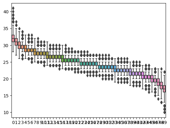
Our response to this challenge of data visualization is to replace each column of dots by a box-and-whiskers plot showing the distribution of the \(i\)-th degree in the sequence. This is done by the following code, and now we will run this on \(10,000\) samples instead of only \(1,000\text{.}\) We will use the pandas and seaborn packages for Python for the data visualization. Unfortunately, Sagecell does not provide enough computational support for this, but if you would like to run additional experiments you can run it at https://cocalc.com/ or through a local Sagemath install.
import pandas as pd
import seaborn as sns

n = 50

p = 0.5

sample_size = 10000

degree_sequences = []

for _ in range(sample_size):
    G = graphs.RandomGNP(n,p)
    seq = sorted(G.degree_sequence())
    seq.reverse()
    degree_sequences.append(seq)

data = pd.DataFrame(degree_sequences,columns=range(n))
ax = sns.boxplot(data=data)
Figure7.1.5.Boxplots for the degree sequence sample.
Note that for the largest degree (the value of \(d_0\) in this code, for which the boxplot is on the far left), the distribution is centered at \(32\text{,}\) which matches our earlier experimental data. These box-and-whisker plots strongly suggest that the typical degree sequence of a graph sampled from \(G(50,0.5)\) passes through a very narrow range of values.
This plot shows that the average value of the eighth-largest degree of a graph in our sample is \(27\text{.}\) Does this make sense to you from the plot above?
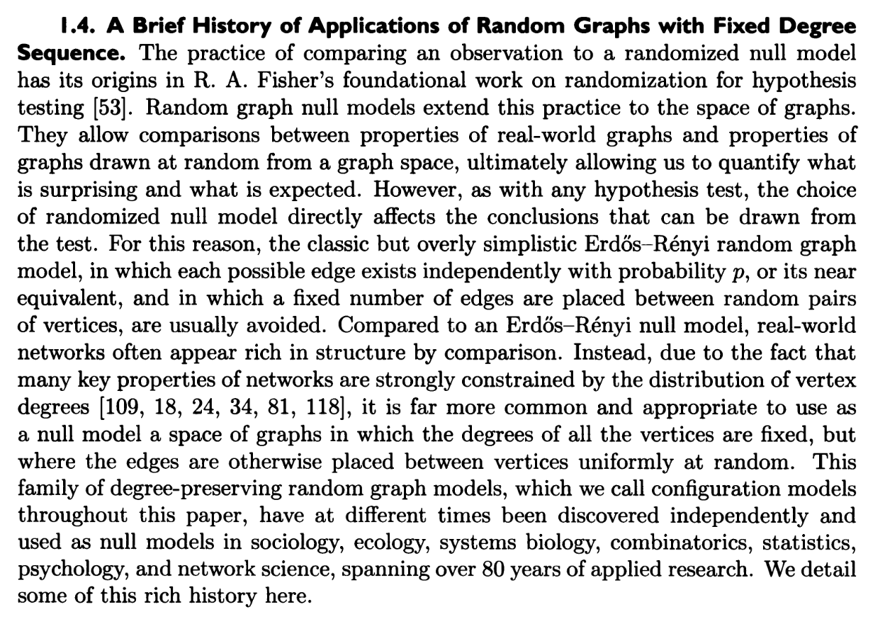
The problem with sampling from an Erdos-Renyi graph is exactly the bias toward certain structural qualities of the graph, which is caused by the underlying binomial distribution. This is articulated clearly in the following quote from Bailey K. Fosdick, Daniel B. Larremore, Joel Nishimura, and Johan Ugander in "Configuring Random Graph Models with Fixed Degree Sequences," SIAM Review 60, no. 2 (2018): 315-55. http://www.jstor.org/stable/45109418
Figure7.1.7.Quote regarding sampling from graph models.
Thus, to sample graphs that have a degree distribution with a different shape than those produced by Erdos-Renyi graphs, we want to sample from either the configuration model we defined previously or one of the many variants of this model. We will consider some experiments using random graphs with a fixed degree sequence generated with almost the uniform distribution, using an algorithm from: Bayati, M., Kim, J.H. & Saberi, A. A Sequential Algorithm for Generating Random Graphs. Algorithmica 58, 860-910 (2010). https://doi.org/10.1007/s00453-009-9340-1 This is called using the Python Networkx package as random_degree_sequence_graph 1
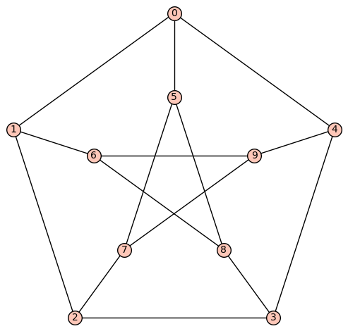
Note that we will no longer be looking at measurements related to the degree sequence, because we have fixed it. However, we might now look at something like number of spanning trees. The following code will generate \(3,000\) random graphs with \(20\) vertices, where each vertex is of degree \(3\text{,}\) to evaluate in https://sagecell.sagemath.org/. It will compute the number of spanning trees for each graph in our sample, show an example of the first graph sampled, and display a histogram of the spanning tree counts for these \(3,000\) graphs.
import networkx as nx
import numpy

sample_size = 3000

spanning_tree_counts = []

for j in range(sample_size):
    G = Graph(nx.random_degree_sequence_graph(20*[3])).copy(immutable=True)
    if j == 0:
        G.show(layout='circular')
        print("number of spanning trees for this graph is: "+str(G.spanning_trees_count()))
    spanning_tree_counts.append(G.spanning_trees_count())

print("mean is: "+str(numpy.mean(spanning_tree_counts)))
print("standard deviation is: "+str(numpy.std(spanning_tree_counts)))
show(histogram(spanning_tree_counts,bins=30))
Note that the average number of spanning trees in a graph in our sample from this model is around \(3.6\)-\(3.8\) million, and the standard deviation is around \(0.9\)-\(1.0\) million. Thus, there is a wide variety of behavior in terms of the number of spanning trees for graphs with \(20\) vertices of degree \(3\text{,}\) and these are graphs that you will probably never sample using the Erdos-Renyi model.
If the number of spanning trees seems large for these graphs, keep in mind that for a graph with \(20\) vertices each having degree \(3\text{,}\) such a graph has \(30\) edges. A tree on such a graph has \(19\) edges. Thus, there are \(\binom{30}{19}=54,627,300\) sets of \(19\) edges in one of these graphs. Our experimental data is suggesting that, on average, the fraction of such sets that form a spanning tree is
We can do a very coarse estimate to compare this with what we know about the Erdos-Renyi model and our computations of expected value. In \(G(20,0.5)\) the expected average degree is \(p(n-1)=\frac{19}{2}=9.5\text{,}\) which is significantly higher than \(3\text{.}\) The expected number of edges is \(p\binom{n}{2}=\frac{1}{2}\binom{20}{2}=95\) and thus in a typical graph the number of subsets with \(19\) edges is approximately
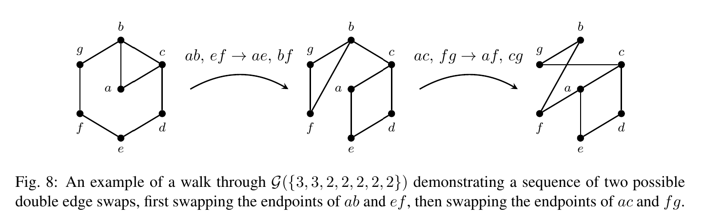
A technique for sampling from connected, loopless, simple (no multiple edges) graphs with a fixed degree sequence is to use Markov Chain Monte Carlo simulation. This is done as follows. Define the graph of graphs \(\mathcal{G}(\mathbf{d})\) to be the directed graph with vertex set all connected graphs with degree sequence \(\mathbf{d}\text{.}\) A connected graph \(G\) has an arrow to \(G'\) in \(\mathcal{G}(\mathbf{d})\) if \(G'\) is obtained from \(G\) via a double-edge swap, i.e., if there exist edges \(uv\) and \(xy\) in \(G\) such that replacing these edges with \(ux\) and \(vy\) produces \(G'\text{.}\)
Figure7.1.9.Figure showing a double-edge swap, taken from: Benjamin Braun, Kaitlin Bruegge, Matthew Kahle. "Facets of Random Symmetric Edge Polytopes, Degree Sequences, and Clustering", Discrete Mathematics & Theoretical Computer Science, December 11, 2023, vol. 25:2.
If performing a particular double-edge swap on \(G\) would produce a graph that is outside the space (i.e. the new graph has a loop or multiedge or is disconnected), that swap will correspond to a loop on the vertex \(G\) in \(\mathcal{G}(\mathbf{d})\text{.}\) It is shown in the paper by Fosdick et. al. referenced above that \(\mathcal{G}(\mathbf{d})\) is regular, strongly connected, and aperiodic, which means that samples asymptotically obey a uniform distribution.
So, to sample using double-edge swaps, one would first create a graph with the degree sequence you want using the reverse of the Havel-Hakimi process. Then, one would repeatedly do random double-edge swaps to produce a "random walk" through the graph.
Starting with the Petersen graph, do a sequence (by hand) of double-edge swaps to sample from the space of finite simple graphs with degree sequence \((3,3,3,3,3,3,3,3,3,3)\text{.}\)