Expected Values: Graphs

Section 4.6 Expected Values: Graphs

We next apply the tools we have developed to investigate expected values of random variables defined on random graphs. We begin with the Erdos-Renyi random graph model \(G(n,p)\text{,}\) which is defined as follows.

🔗

Definition 4.6.1.

Let \(n\) be a positive integer and \(p\) be a real number with \(0 \lt p \lt 1\text{.}\) The Erdos-Renyi random graph model \(G(n,p)\) is the probability space whose set of events consists of all graphs with vertex set \(\{1,2,\ldots,n\}\text{,}\) where each edge is included independently with probability \(p\text{.}\) Thus, the probability of a particular graph \(G\) with \(e\) edges is \(p^e (1-p)^{\binom{n}{2}-e}\text{.}\)

🔗

The Erdos-Renyi model is one of the most well-studied random graph models. It is actually a binomial distribution in disguise, since it is equivalent to considering binary strings of length \(\binom{n}{2}\text{,}\) where each bit corresponds to the presence or absence of a particular edge, as the following example illustrates.

🔗

Example 4.6.2.

Let \(n=4\) and \(p=\frac{1}{2}\text{.}\) Then the probability space \(G(4,\frac{1}{2})\) consists of all graphs with vertex set \(\{1,2,3,4\}\text{,}\) where each edge is included independently with probability \(\frac{1}{2}\text{.}\) There are \(\binom{4}{2}=6\) possible edges, so there are \(2^6=64\) possible graphs in this model, each with probability \(\left(\frac{1}{2}\right)^6=\frac{1}{64}\text{.}\) Thus, this model gives the uniform distribution on the set of all graphs with vertex set \(\{1,2,3,4\}\text{.}\) Further, each graph can be represented by a binary string of length \(6\text{,}\) where we index the entries of the string by the edges \(12, 13, 14, 23, 24, 34\text{.}\) Then, the entry is \(1\) if the corresponding edge is present, and \(0\) otherwise. For example, the graph with edges \(12\text{,}\) \(14,\) and \(23\) corresponds to the binary string \(101100\text{.}\)

🔗

Using this connection to the binomial distribution, we can compute expected values of various graph statistics in the Erdos-Renyi model. We illustrate this with the following theorem.

🔗

Theorem 4.6.3.

The expected number of edges in a graph drawn from the Erdos-Renyi model \(G(n,p)\) is \(p \binom{n}{2}\text{.}\)

🔗

Proof.

Using the fact that \(G(n,p)\) is equivalent to a binomial distribution on binary strings of length \(\binom{n}{2}\) and probability \(p\text{,}\) we have that the expected number of edges is \(p \binom{n}{2}\text{.}\)

🔗

We can also investigate properties of Erdos-Renyi graphs that do not immediately make sense for only binary strings. This is because binary strings do not have an automatic relationship between the different positions in the string, but graphs do via their vertices and edges, and the binary strings corresponding to graphs in the Erdos-Renyi model respect this structure.

🔗

Theorem 4.6.4.

The expected number of isolated vertices in a graph drawn from the Erdos-Renyi model \(G(n,p)\) is \(n(1-p)^{n-1}\text{.}\)

🔗

Proof.

Let \(X\) be the random variable giving the number of isolated vertices in a graph drawn from \(G(n,p)\text{.}\) For \(1 \leq i \leq n\text{,}\) let \(X_i\) be the indicator random variable for the event that vertex \(i\) is isolated. Then we have

\begin{equation*} X = X_1 + X_2 + \cdots + X_n. \end{equation*}

By linearity of expectation, we have

\begin{equation*} E[X] = E[X_1] + E[X_2] + \cdots + E[X_n]. \end{equation*}

Now, for each \(i\text{,}\) we have

\begin{equation*} E[X_i] = P(X_i = 1) = (1-p)^{n-1}, \end{equation*}

since for vertex \(i\) to be isolated, none of the \(n-1\) edges connecting it to the other vertices can be present, and each edge is absent with probability \(1-p\text{.}\) Thus, we have

\begin{equation*} E[X] = n(1-p)^{n-1}. \end{equation*}

🔗

Checkpoint 4.6.5.

Discuss the proof above. Does it make sense? Why or why not?

🔗

We can also compute the expected number of triangles, i.e., the number of \(K_3\)’s, in an Erdos-Renyi graph.

🔗

Theorem 4.6.6.

Let \(X\) be the random variable giving the number of triangles in a graph drawn from the Erdos-Renyi model \(G(n,p)\text{.}\) Then

\begin{equation*} E[X]=\binom{n}{3} p^3 \, . \end{equation*}

🔗

Proof.

Let \(X\) be the random variable giving the number of triangles in a graph drawn from \(G(n,p)\text{.}\) For \(1 \leq i \lt j \lt k \leq n\text{,}\) let \(X_{i,j,k}\) be the indicator random variable for the event that the vertices \(i, j, k\) form a triangle, i.e., that the edges \(\{i,j\},\{i,k\},\{j,k\}\) are all present in the graph. Then we have

\begin{equation*} X = \sum_{1 \leq i \lt j \lt k \leq n} X_{i,j,k}. \end{equation*}

By linearity of expectation, we have

\begin{equation*} E[X] = \sum_{1 \leq i \lt j \lt k \leq n} E[X_{i,j,k}]. \end{equation*}

Now, for each triple \((i,j,k)\text{,}\) we have

\begin{equation*} E[X_{i,j,k}] = P(X_{i,j,k} = 1) = p^3, \end{equation*}

since for vertices \(i, j, k\) to form a triangle, all three edges connecting them must be present, and each edge is present with probability \(p\text{.}\) Thus, we have

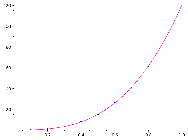
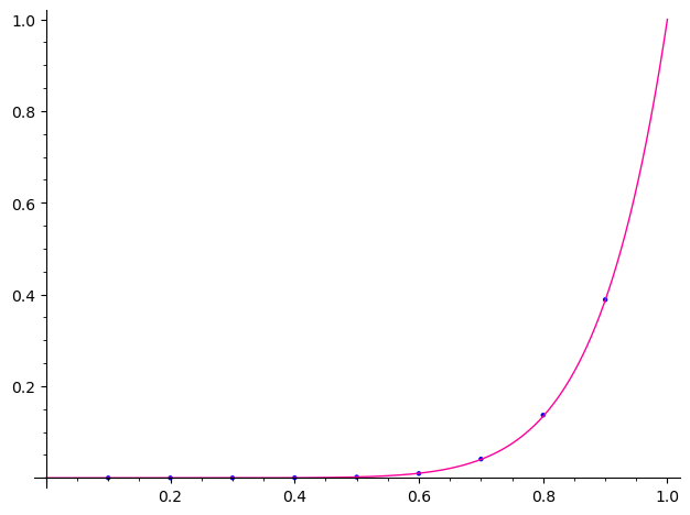
\begin{equation*} E[X] = \binom{n}{3} p^3. \end{equation*}

🔗

Checkpoint 4.6.7.

Discuss the proof above. Does it make sense? Why or why not?

🔗

It is good to get in the habit of checking whether your expected value results make sense. For example, in the last theorem, as \(p\) approaches \(0\text{,}\) the expected number of triangles approaches \(0\text{,}\) which makes sense since there are fewer edges in the graph. Similarly, as \(p\) approaches \(1\text{,}\) the expected number of triangles approaches \(\binom{n}{3}\text{,}\) which makes sense since the graph is approaching the complete graph \(K_n\text{,}\) which has \(\binom{n}{3}\) triangles.

🔗

We can also get in the habit of comparing our expected value results to actual values obtained from simulations. For example, we can simulate drawing graphs from \(G(10, p)\) and counting the number of triangles in each graph. Doing this for various values of \(p\) should give values close to those predicted by our theorem. Note that

\begin{equation*} \binom{10}{3} = 120\text{,} \end{equation*}

so the expected number of triangles in \(G(10,p)\) is \(120 p^3\text{.}\) How does this compare to simulations where we randomly generate \(1000\) graphs from \(G(10,p)\) for \(p=0.1,0.2,\ldots , 0.9\) and compute the average number of triangles per graph for each sample?

🔗

Plot of experimental expected value of number of triangles versus p. — Figure 4.6.8. Plot of experimental expected value of number of triangles versus \(p\) overlaid with the plot of \(y=\binom{10}{3}p^3\text{.}\)
🔗

Checkpoint 4.6.9.

Discuss the simulation results above. Do they make sense? Why or why not?

🔗

Let’s look at two more examples of computing expected values in the Erdos-Renyi model. First, we will consider the expected average degree of a vertex.

🔗

Theorem 4.6.10.

Let \(X\) be the random variable giving the average degree of a vertex in a graph drawn from the Erdos-Renyi model \(G(n,p)\text{.}\) Then

\begin{equation*} E[X]=p(n-1)\text{.} \end{equation*}

🔗

Proof.

Let \(X\) be the random variable giving the average degree of a vertex in a graph drawn from \(G(n,p)\text{.}\) By definition, we have

\begin{equation*} X = \frac{\deg(1) + \deg(2) + \cdots + \deg(n)}{n}, \end{equation*}

where \(\deg(i)\) is the degree of vertex \(i\text{.}\) By linearity of expectation, we have

\begin{equation*} E[X] = \frac{E[\deg(1)] + E[\deg(2)] + \cdots + E[\deg(n)]}{n}. \end{equation*}

Now, for each \(i\text{,}\) we have

\begin{equation*} E[\deg(i)] = p(n-1), \end{equation*}

since the degree of vertex \(i\) is the sum of \(n-1\) indicator random variables for the presence of each edge connecting vertex \(i\) to the other vertices, each of which has expected value \(p\text{.}\) Thus, we have

\begin{equation*} E[X] = p(n-1). \end{equation*}

🔗

Checkpoint 4.6.11.

Discuss the proof above. Does it make sense? Why or why not?

🔗

As our final example, we will find the expected number of spanning trees in an Erdos-Renyi graph.

🔗

Theorem 4.6.12.

Let \(T\) be the random variable giving the number of spanning trees in a graph drawn from the Erdos-Renyi model \(G(n,p)\text{.}\) Then

\begin{equation*} E[T]=p^{n-1} n^{n-2}\text{.} \end{equation*}

🔗

Proof.

Let \(T\) be the random variable giving the number of spanning trees in a graph drawn from \(G(n,p)\text{.}\) For each spanning tree \(S\) on vertex set \(\{1,2,\ldots,n\}\text{,}\) let \(T_S\) be the indicator random variable for the event that spanning tree \(S\) is present in the graph. Then we have

\begin{equation*} T = \sum_{S} T_S, \end{equation*}

where the sum is over all spanning trees \(S\) on vertex set \(\{1,2,\ldots,n\}\text{.}\) By linearity of expectation, we have

\begin{equation*} E[T] = \sum_{S} E[T_S]. \end{equation*}

Now, for each spanning tree \(S\text{,}\) we have

\begin{equation*} E[T_S] = P(T_S = 1) = p^{n-1}, \end{equation*}

since a spanning tree on \(n\) vertices has \(n-1\) edges, and each edge is present with probability \(p\text{.}\) By Cayley’s formula, there are \(n^{n-2}\) spanning trees on vertex set \(\{1,2,\ldots,n\}\text{.}\) Thus, we have

\begin{equation*} E[T] = p^{n-1} n^{n-2}. \end{equation*}

🔗

Checkpoint 4.6.13.

Discuss the proof above. Does it make sense? Why or why not?

🔗

Let’s do one final check to see if this result makes sense. As \(p\) approaches \(0\text{,}\) the expected number of spanning trees approaches \(0\text{,}\) which makes sense since there are fewer edges in the graph. Similarly, as \(p\) approaches \(1\text{,}\) the expected number of spanning trees approaches \(n^{n-2}\text{,}\) which makes sense since the graph is approaching the complete graph \(K_n\text{,}\) which has \(n^{n-2}\) spanning trees by Cayley’s formula. Finally, we can simulate drawing graphs from \(G(10, p)\) and counting the number of spanning trees in each graph, as we did for triangles above.

🔗

Plot of experimental expected value of number of spanning trees versus p overlaid with the plot of y=10^8p^9. — Figure 4.6.14. Plot of experimental expected value of number of spanning trees versus \(p\) overlaid with the plot of \(y=10^8p^9\text{.}\)
🔗

🔗

Prev Top Next