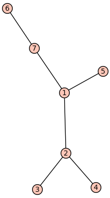
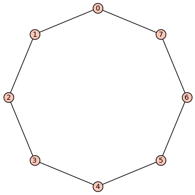
MA 415G course notes

Section 3.5 Prufer Codes and Cayleyโ€™s Theorem

Our next classification goal is to classify all labeled trees on \(n\) vertices. This is an example of classifying the spanning trees in the complete graph, defined as follows.

Definition 3.5.1.

Given a finite connected graph \(G\text{,}\) a spanning tree of \(G\) is a tree \(T\) on the same vertex set as \(G\) where the edge set of \(T\) is contained in the edge set of \(G\text{,}\) i.e., \(E(T)\subseteq E(G)\text{.}\)

Example 3.5.2.

The cycle graph on \(n\) vertices, denoted \(C_n\text{,}\) is the graph on vertex set \([n]\) with edge set
\begin{equation*} \{\{1,2\},\{2,3\},\{3,4\},\ldots,\{n-1,n\},\{n,1\}\} \, . \end{equation*}
In the following example, we have shown \(C_8\) using the vertex set \(\{0,1,2,3,4,5,6,7\}\text{.}\) If we remove any edge from \(C_8\text{,}\) the resulting graph is a spanning tree. Thus, there are eight spanning trees of \(C_8\text{.}\)
Figure 3.5.3. Example of \(C_8\text{.}\)
Note that for our purposes, we considered spanning trees to be distinct when they are different as labeled graphs. So, in our example of \(C_8\) above, even though every spanning tree was a path with seven edges, they are all considered distinct because they each have a unique vertex labeling.

Checkpoint 3.5.4.

Systematically list all the labeled spanning trees of \(K_n\) for \(n=2,3,4,5\text{.}\) Write the vertex set of \(K_n\) as \(\{0,1,2,\ldots,n-1\}\text{.}\)
Figure 3.5.5. Example of \(K_5\text{.}\)
The sequence \(n^{n-2}\) for \(n\geq 2\) is given by
\begin{equation*} 1, 3, 16, 125, 1296, 16807, 262144, 4782969, 100000000, 2357947691,\ldots \end{equation*}
and is found in the Online Encyclopedia of Integer Sequences as https://oeis.org/A000272.

Checkpoint 3.5.7.

Discuss with your group: suppose that you generated the first few values of this sequence by listing the spanning trees of \(K_n\) and realized that it matched \(n^{n-2}\text{.}\) What would you do next? What are some different strategies you could use to approach the problem of showing that your conjectured formula is correct?
There are multiple strategies for proving that this formula is correct, including:
  • Using the technique of exponential generating functions to compute this value algebraically. The downside to this technique is it gives you the formula but without a combinatorial proof.
  • Apply the matrix-tree theorem, which gives a matrix-algebra based technique for computing the number of spanning trees in a graph using determinants. This is based on 19th century techniques due to Kirchoff using the Laplacian matrix of a graph, which is a discrete model for heat flow through a network.
  • Double-counting, where one counts the same object in two different ways. You used this technique on the homework to prove that \(\binom{n}{k}=\frac{n!}{k!(n-k)!}\text{.}\)
  • A bijective approach, where we find a set of size \(n^{n-2}\) and find an explicit bijection between that set and the spanning trees of \(K_n\text{.}\)
We will use a bijective approach to prove Cayleyโ€™s Theorem.

Checkpoint 3.5.8.

Proof of Theoremย 3.5.6.

By Theoremย 3.5.9, we have that the number of spanning trees of \(K_n\) is the same as the number of sequences in \([n]^{n-2}\text{,}\) which is \(n^{n-2}\text{.}\)
What remains is for us to prove Theoremย 3.5.9, i.e., to prove that we have such a bijection.

Definition 3.5.10.

Suppose \(T\) is a spanning tree of \(K_n\) on vertex set \([n]\text{.}\) We construct an array
\begin{equation*} A(T):= \begin{bmatrix} x_1 \amp x_2 \amp \cdots \amp x_{n-1} \\ y_1 \amp y_2 \amp \cdots \amp y_{n-1} \end{bmatrix} \end{equation*}
as follows:
  1. Set \(T_1:=T\text{.}\) Let \(x_1\) be the leaf of \(T\) with the smallest label, with neighbor \(y_1\text{.}\) Remove \(x_1\) and the edge \(\{x_1,y_1\}\) from \(T_1\) to create a new tree \(T_2\text{,}\) and place those vertex labels as the first column in the array.
  2. Let \(x_2\) be the leaf of \(T_2\) with the smallest label, with neighbor \(y_2\text{.}\) Remove \(x_2\) and the edge \(\{x_2,y_2\}\) from \(T_2\) to create a new tree \(T_3\text{,}\) and place those vertex labels as the second column in the array.
  3. Let \(x_3\) be the leaf of \(T_3\) with the smallest label, with neighbor \(y_3\text{.}\) Remove \(x_3\) and the edge \(\{x_3,y_3\}\) from \(T_3\) to create a new tree \(T_4\text{,}\) and place those vertex labels as the third column in the array.
  4. Continue in this manner until all edges of \(T\) have been removed.
Recall that there are \(n-1\) edges in \(T\) and every tree has at least one leaf. Therefore, this algorithm will terminate and result in a matrix of the form \(A(T)\text{.}\)
The Prufer code for \(T\) is the vector \(P(T):=(y_1,y_2,y_3,\ldots,y_{n-2})\in [n]^{n-2}\text{.}\)

Checkpoint 3.5.11.

Show that the Prufer code for the following tree is given by \((2,2,1,1,7)\text{.}\)
Figure 3.5.12. Tree for Prufer code exercise.

Proof of Theoremย 3.5.9.

We will prove Theoremย 3.5.9 by showing that the Prufer code function is invertible. If the map \(P\) sending spanning trees to sequences in \([n]^{n-2}\) has an inverse, then it is both one-to-one and onto, hence it is a bijection.
Consider the following algorithm, applied to a sequence \(y=(y_1,\ldots,y_{n-2})\in [n]^{n-2}\) to produce a tree \(R(y)\text{.}\) Start with an empty graph \(T_0\text{.}\)
  1. Consider the smallest element of \([n]\) that is not listed in \(y\text{.}\) Call this element \(x_1\) and add the edge \(\{x_1,y_1\}\) to \(T_0\) to create \(T_1\text{.}\) Delete \(y_1\) from \(y\text{.}\)
  2. Consider the smallest element of \([n]\setminus \{x_1\}\) that is not listed in \((y_2,\ldots,y_{n-2})\text{.}\) Call this element \(x_2\) and add the edge \(\{x_2,y_2\}\) to \(T_1\) to create \(T_2\text{.}\) Delete \(y_2\) from \(y\text{.}\)
  3. Consider the smallest element of \([n]\setminus \{x_1,x_2\}\) that is not listed in \((y_3,\ldots,y_{n-2})\text{.}\) Call this element \(x_3\) and add the edge \(\{x_3,y_3\}\) to \(T_2\) to create \(T_3\text{.}\) Delete \(y_3\) from \(y\text{.}\)
  4. Continue in this fashion until you have created a tree \(T\) with \(n-1\) edges.
We have that \(R(P(T))=T\) by construction, and therefore we have that \(R=P^{-1}\text{,}\) as desired.

Checkpoint 3.5.13.

Show that the Prufer code \((2,2,1,1,7)\) builds the following tree.
Figure 3.5.14. Tree for second Prufer code exercise.

Checkpoint 3.5.15.

Create the tree \(T\) corresponding to the Prufer code \((1,3,2,4,3,3,3)\) and then verify that \(P(T)\) is equal to this code.

Checkpoint 3.5.16.

Discuss with your group why it is that \(R=P^{-1}\text{.}\) Does this make sense? Why or why not?

Proof.

If \(j\) is a leaf of \(T\text{,}\) then it will only appear in a column of the array for \(T\) when it is the smallest labeled leaf in a tree during the Prufer code algorithm. Thus, \(j\) will only appear in the top row of the array, not the bottom row.
For every vertex \(i\) that is not a leaf of \(T\text{,}\) it will appear as the lower-column-entry in the array for edges until \(i\) is the least-labeled leaf in one of the trees appearing in the algorithm. Thus, \(i\) will appear in the Prufer code \(\deg_T(i)-1\) many times, as it will not become a leaf until it has had enough edges removed so that it has degree \(1\) in a tree arising in the Prufer code algorithm.

Checkpoint 3.5.18.

Check the argument from this proof using the checkpoint examples above.